ETOOBUSY 🚀 minimal blogging for the impatient
A Quest for Voronoi Diagrams - 2. Fortune's Implementation
In the first article about my quest for Voronoi diagrams I ranted a bit about how everybody around seems to be talking about Fortune’s algorithm without having bothered to read Steven Fortune’s paper from 1987 A sweepline algorithm for Voronoi diagrams.
Fortune also implemented the algorithm described in the paper as a C program. It does what’s written on the can and more, so it’s not exactly straightforward to follow.
I’ll put some notes below about what I understood of it… I hope they can be useful. The code can be found in Fortune’s homepage (here a link to the copy at the Internet Archive).
Adherence To The Paper
The program is largely adherent to the paper, with some caveats:
-
the priority queue $Q$ is implemented in a “split arrangement” where sites and vertices are kept separated (actually, only the latter ones end up in a real priority queue). This is an implementation trick that, to any extent, is totally equivalent to having a single queue;
-
the sequence $L$ of $(r_1, c_1, r_2, …, r_k)$ of regions and boundaries is implemented as a doubly-linked list of branches only, where branches carry around also information about their associated regions. From a representation point of view it’s equivalent, but…
-
a doubly-linked list for branches cannot be used for a binary search of the “right” region, which somehow defies the complexity analysis, although Fortune also implements a hash-based indexing of the doubly-linked list that improves performance (I have no idea about the asymptotic complexity though).
Data Structures
The data structures used in the implementation can be divided into two main categories:
- basic
structs/types:Point,Site,Edge,Halfedge. These are defined insidevdefs.h(ordefs.hin some implementations); - more complex data structures, like the Priority Queue and the Edge List. Their definition/implementation is not found in a single place.
Some additional structures/types are also introduced to enhance memory management, but they will not be discussed here.
Point
The definition of type Point is as simple as it can get, just a place
to keep track of x and y coordinates:
typedef struct tagPoint
    {
    float x ;
    float y ;
    } Point ;
Site
A Site is slightly more than a Point:
typedef struct tagSite
    {
    Point coord ;
    int sitenbr ;
    int refcnt ;
    } Site ;
One aspect is that sitenbr provides an identity to the specific
Point coord, like a label or a tag. The refcnt helps with memory
management and optimization, so it can be ignored from the sweeping line
algorithm’s point of view.
The Site type is used to represent both sites and vertices. While
this choice might be considered cheap when coming from higher
abstraction level languages, this is C and using the same type for
entities that share a common fate (the extraction from the Priority
Queue can yield either a site or a vertex) is a solid design
decision. If anything, I would have probably called it something like
Place to avoid a possible misunderstanding.
Edge
An Edge represents a bisector line in the plane, with some strings
attached. With reference to the article, it represents a boundary
between two sites, i.e. $B_{pq}$ (if sites are p and q).
typedef struct tagEdge
    {
    float a, b, c ;
    Site * ep[2] ;
    Site * reg[2] ;
    int edgenbr ;
    } Edge ;
Floats a, b and c are coefficients for the line, according to the
following equation:
When a new Edge is created by function bisect in geometry.c,
the parameters are normalized so that either a or b is forced to
1. In particular, more vertical lines have a set to 1, while
more horizontal lines have b set to 1, which is consistent with
fully vertical or horizontal where b and a would be 0,
respectively. This also means that a and b are, in absolute value,
always less than or equal to 1.
The two-slots array of pointers to Site named reg holds pointers
towards the two sites that define the bisector. These are real input
sites: a bisector always cuts the plane in two halves, each containing
the points that are closer to one of the two sites. In the article’s
formalism, if $B_{pq}$ is the boundary, reg holds pointers to Sites
p and q.
When a new Edge is created in bisect@geometry.c, the lower or
leftier site is always put first and the higher or righter site
second. This means that the first slot contains the pointer to the site
that is either at lower y coordinate or, if the two sites have the same
y coordinate, at lower x coordinate. The definition of the following
macros:
#define le 0
#define re 1
also assigns a semantic to these slots: the bottom site is considered to
be on the left, the other one on the right. This gives the Edge a
natural orientation that always goes from right to left, as shown in the
following picture.
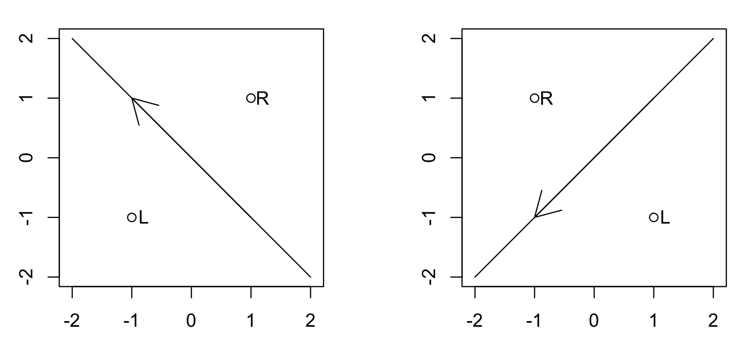
Every Edge created by bisect@geometry.c has two sites in reg. On
the other hand, you might hit a null Edge that is actually a NULL
pointer, representing a line at infinity.
The two-slots array of pointers to Site named ep, on the other hand,
holds optional pointers to vertices. The optionality is given both
by intrinsic reasons (e.g. collinear sites give raise to parallel edges
with no vertices, and all edges at the boundary only have one vertex
as endpoint but go to infinity otherwise) or algorithm phase reasons
(e.g. a vertex has not been introduced yet).
Last, edgenbr provides a unique identity to the Edge, so that if the
same line arises again the two resulting edges can be distinguished.
Halfedge
In the original article, each edge $B_{pq}$ (assuming p is “greater
than” q as per previous section) is divided into two pieces, namely
$C^-_{pq}$ (that lies left of p) and $C^+_{pq}$ (that lies right of p).
The Halfedge represents one such part.
#define le 0
#define re 1

typedef struct tagHalfedge
    {
    struct tagHalfedge * ELleft ;
    struct tagHalfedge * ELright ;
    Edge * ELedge ;
    int ELrefcnt ;
    char ELpm ;
    Site * vertex ;
    float ystar ;
    struct tagHalfedge * PQnext ;
    } Halfedge ;
This structure mixes in the same place aspects that belong to different operations and semantics.
The real representation of an edge’s halves $C^-_{pq}$ and $C^+_{pq}$ is in the following members:
ELedgepoints to the edge/bisector that thisHalfedgeis part of. This might be aNULLpointer, in which case theHalfedgerepresents a part of a boundary at the infinite (ideally, the boundary between the bottomest site and a site at infinite). The ordering of the twoSitepointers inreginsideELedgeallows understanding which is p (the one on the right/second slot) and which is q (the one on the left/first slot).ELpmindicates whether this is the minus/left (i.e. $C^-_{pq}$) or the plus/right (i.e. $C^+_{pq}$) part of the edge. It takes valuele(macro for0) for the left part andre(macro for1) for the right part.
Other members have to do with the fact that Halfedge triples down as
the central structure for representing the Edges List and the Priority
Queue too. In particular:
- the Edge List is basically represented as a double-linked list, hence
ELleftandELrightare pointers to the nearbyHalfedges; - the Priority Queue contains also vertices, hence the members:
vertexis an optional pointer to a vertex, populated in case thisHalfedgecrosses a nearby pre-existingHalfedgeat the time of its creation.ystarrepresents the y coordinate in the*-transformed space of thevertex, if any.PQnextis the next vertex-bearingHalfedgein vertical ascending order, if any.
Last, member ELrefcnt is there for memory allocation optimization and
will be ignored in the rest of this post.
The Priority Queue
The Priority Queue described in the article’s algorithm implements an efficient mechanism to determine the next notable point hit by the sweepline, i.e. either a site (leading to a site event) or a vertex (leading to a vertex event).
Theoretically, these would be homogeneous elements put in the same Priority Queue $Q$ data structure. From an implementation point of view, though, the $Q$ is implemented in a half-implicit way as follows:
-
all sites are known beforehand and initially sorted (either externally or by the program itself). The array is iterated in
voronoi.cusing functionnextsite, that is provided as input. This is an implementation trick that allows passing an already sorted list in a file and avoid doing the sorting again (as well as reading the whole list in memory); -
all vertices are discovered along the way and kept in a sub Priority Queue. As a matter of fact, this contains
Halfedges, because they contain a pointer to a vertex, which also accounts for the presence of memberPQnextinHalfedge. The implementation of this sub Priority Queue is through a heap and the associated method-like functions can be found inheap.c. -
The overall implementation is in
voronoi.cand, in particular, in the way that events are extracted. At each iteration, the bottomest site is compared against the bottomest vertex (in this case, usingHalfedge’s memberystar, because the sweepline “lives” in the*-transformed space) and the lower one is processed, leading to either a site event or to a vertex event just like the two different kinds of places were all put together in a single Priority Queue.
The Edge List
The list described in the algorithm is supposed to contain a sequence of
*-transformed regions and boundaries, where boundaries are ordered by
x coordinate and regions can appear multiple times.
In the implementation, the Edge List only contains Halfedges, i.e.
parts of the boundaries, and the associated regions can be deduced by
looking at the boundaries (at the end of the day, a $C^-_{pq}$
Halfedge has p on the left side and q on the right side).
For this reason, it is kept as a doubly-linked list of Halfedges; to
make the implementation more compact, the machinery for the
doubly-linked list is drown inside Halfedge itself, leading to members
ELleft and ELright.
There is more to this though. Using a simple doubly-linked list would
defy the algorithm’s claim of $n \cdot log(n)$ complexity, because
iterating through it would take $n$ time instead of $log(n)$. Ideally,
this should be implemented with a data structure that allows binary
searching over the list of Halfedges (which would be possible thanks
to the fact that they can be sorted on the x axis).
For this reason, an hash-based mechanism is added on top of the
doubly-linked list, to provide more efficient “entry points” in the list
and speed up the search. After finding the most probable spot as a
starting point, the list is searched towards the left or towards the
right (depending on the relative positions) until the right Halfedge
is found. This hash-based mechanism is implemented in edgelist.c,
which also contains the logic for searching the closer boundary on the
left of a Point (ELleftbnd@edgelist.c).
Site Event - The Right Region in V(*)
As already indicated in the first post of the quest, a key part of Fortune’s original algorithm is finding the most interested region by the introduction of a new site.
The algorithm’s description suggests to consider the different sections of hyperbola and how they intersect to find this out, although this is arguably a bit vague. Or, maybe, it’s explained well in the mathematical section but I wasn’t too sharp in understanding it immediately.
Skimming through Halfedges
At the high level, when a new site is found by the sweep line, the
list of all Halfedges found so far is iterated to find the closest one
that immediately on the left of this new site. This is done by function
ELleftbnd in file edgelist.c. It should ideally be a binary search,
as a matter of fact it’s a kind-of linear search optimized with a good
guess on the best entry point in the list, via a hash-like mechanism.
Based on the new site’s position, the function takes a first guess at
where the most realistic candidate might be in the linked list (this is
done using a sort of “hash-cache” pointing to different positions in the
doubly-linked list of Halfedges), then moves left or right depending
on whether the specific Halfedge is on the right of the new site or
not.
One source of doubts when reading the algorithm was the claim that the
list of $(r_1, c_1, r_2, …, r_k)$ is ordered by the x coordinate
while, at the same time, it can contain the same region multiple times.
What I wasn’t grasping is that the ordering is only referred to the
boundary halves, not the regions. This is of course immediate to
understand looking at the following picture, representing the
transformed space.
By keeping only Halfedges in the list, and iterating it using
right_of@geometry.c, the implementation is indeed capable of
leveraging the ordering by x, even though not in the binary search
approach suggested in the article but using the hashing mechanism to
speed up lookups.
How much above is above?
The key to moving or stopping is function right_of implemented in
geometry.c. I initially struggled a bit on this, because its naming of
a few variables can be misleading (in particular, the above variable
was super-confusing for me, but it was all my fault). This leads us to
the following section.
It has to be kept in mind that all operations in the algorithm are
thought to happen in the *-transformed space, hence they take into
account the Voronoi diagram in the transformed space instead of the
original diagram. Thanks to the * transformation introduced by
Fortune, all but the sites are pushed up in the plane, so when
comparing the y coordinate of two points this has to be taken into
account.
The code for right_of@geometry.c makes a distinction based on whether
the edge line is more vertical (i.e. a == 1.0) or horizontal (i.e.
b == 1.0) but, apart from a technical detail regarding totally
vertical lines, the two are equivalent. The latter case establishes
whether the new site is above a Halfedge like this:
else  /*** e->b == 1.0 ***/
    {
    yl = e->c - e->a * p->x ;
    t1 = p->y - yl ;
    t2 = p->x - topsite->coord.x ;
    t3 = yl - topsite->coord.y ;
    above = ((t1*t1) > ((t2 * t2) + (t3 * t3))) ;
    }
We will get shortly to why above helps us understand whether a site
is right_of the Halfedge. My initial confusion is that the code
above compares the distance of the new Site from the point on the
bisector immediately below against the distance of this latter point
from the topsite (it’s easy to spot Pythagora’s theorem in the
inequality).
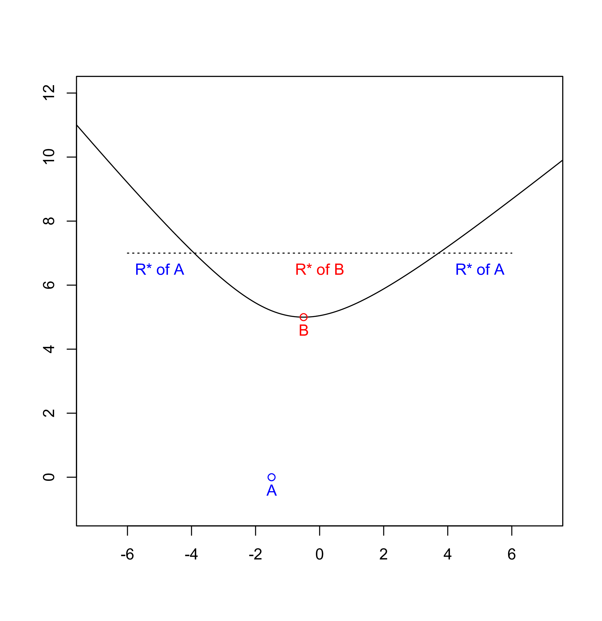
Now consider the following picture as an example.

My eyes tell me that site X would be above the Halfedge, and yet the
algorithm says it isn’t: point V is mapped onto Y by the *
transformation, and X is below it.
This apparent paradox depends on the fact that the picture is not representing what happens in the transformed space, which is what the following picture does.
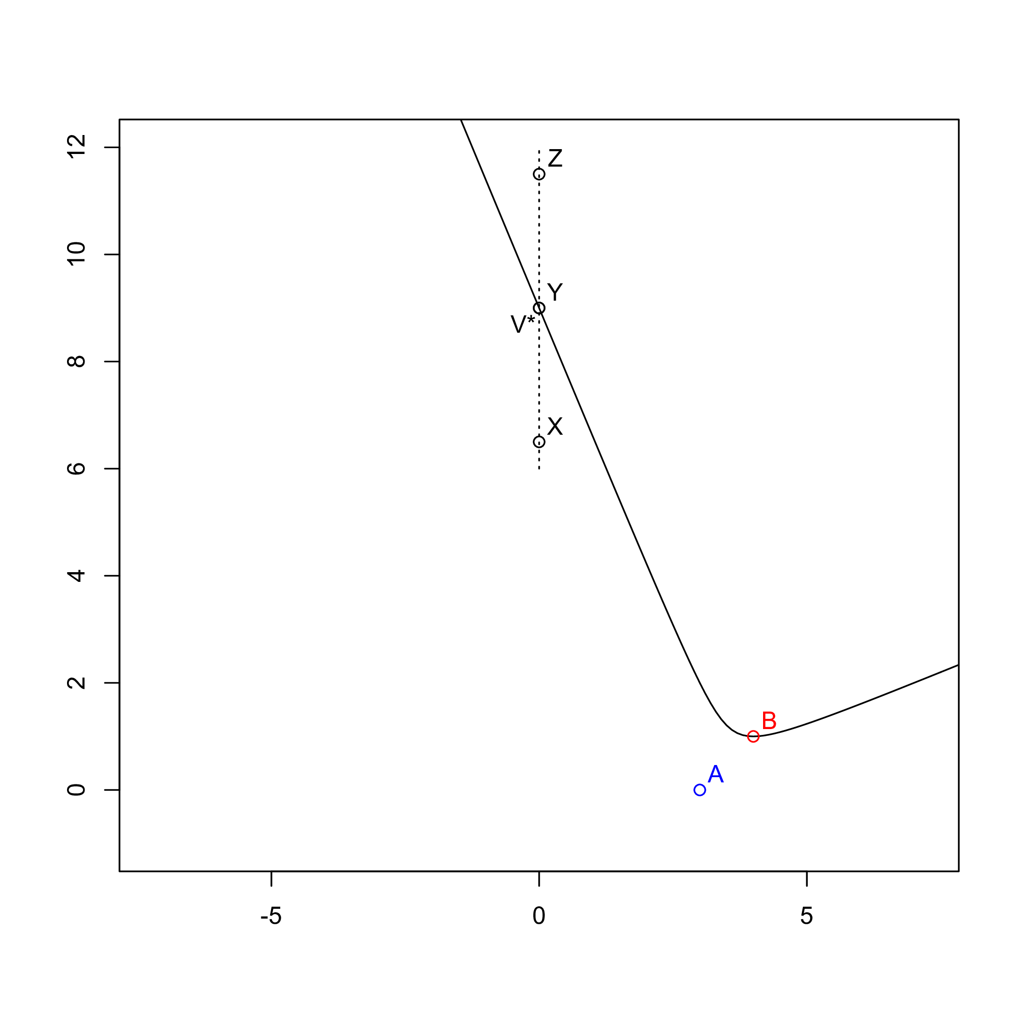
Now it’s indeed clear why X lies below the Halfedge and Z
above it. It’s also easy, at this point, to understand why above can
help us understand whether the new site is left or right of the
Halfedge: below means left (like X) and above means right
(like Z), at least for a left Halfedge (the picture shows the
left Halfedge because it’s left of its base site, i.e. B).
What would happen with a right Halfedge is easily understood from
the following picture though.
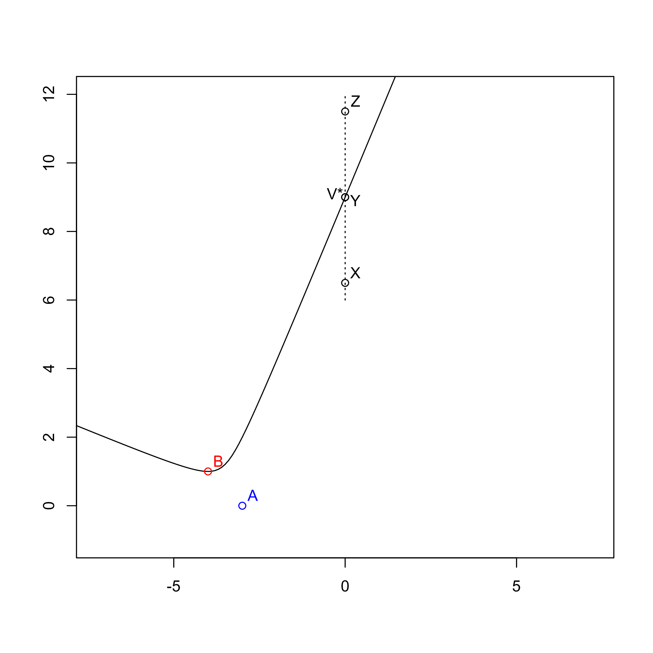
In short, for right Halfedges the relations are inverted: above
means left and below means right. This eventually explains the
return value from function right_of:
return (el->ELpm == le ? above : !above) ;
The condition el->ELpm indicates whether it is a left Halfedge
(the $C^-_{pq}$ part in the algorithm’s description inside the article)
or a right one (the $C^-_{pq}$ part). For left Halfedges, being on
the right is the same as being above, otherwise it’s the contrary
(as we saw before).
Wrap Up
Fortune’s original implementation helps shed a light on the very high-level description of the algorithm provided in the original article from 1987 A sweepline algorithm for Voronoi diagrams, which is also - arguably - the only one that can be called Fortune’s algorithm (at least when linking that paper!).
The implementation is somehow optimized and not really easy to follow, because optimizations (like memory management) are intermixed to enhance performance. Still it’s been very instructive to read it and hopefully understand it as well.